Convolutional networks (ConvNets) currently set the state of the art in visual recognition. The aim of this project is to investigate how the ConvNet depth affects their accuracy in the large-scale image recognition setting.

What is VGG

VGG16 is a convolutional neural network model proposed by K. Simonyan and A. Zisserman from the University of Oxford in the paper “Very Deep Convolutional Networks for Large-Scale Image Recognition”. The model achieves 92.7% top-5 test accuracy in ImageNet, which is a dataset of over 14 million images belonging to 1000 classes. It was one of the famous model submitted to ILSVRC-2014. It makes the improvement over AlexNet by replacing large kernel-sized filters (11 and 5 in the first and second convolutional layer, respectively) with multiple 3×3 kernel-sized filters one after another. VGG16 was trained for weeks and was using NVIDIA Titan Black GPU’s.

The Architecture

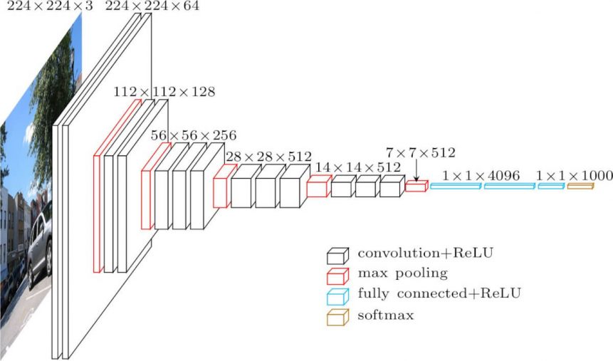
The input to cov1 layer is of fixed size 224 x 224 RGB image. The image is passed through a stack of convolutional (conv.) layers, where the filters were used with a very small receptive field: 3×3 (which is the smallest size to capture the notion of left/right, up/down, center). In one of the configurations, it also utilizes 1×1 convolution filters, which can be seen as a linear transformation of the input channels (followed by non-linearity). The convolution stride is fixed to 1 pixel; the spatial padding of conv. layer input is such that the spatial resolution is preserved after convolution, i.e. the padding is 1-pixel for 3×3 conv. layers. Spatial pooling is carried out by five max-pooling layers, which follow some of the conv. layers (not all the conv. layers are followed by max-pooling). Max-pooling is performed over a 2×2 pixel window, with stride 2.

Three Fully-Connected (FC) layers follow a stack of convolutional layers (which has a different depth in different architectures): the first two have 4096 channels each, the third performs 1000-way ILSVRC classification and thus contains 1000 channels (one for each class). The final layer is the soft-max layer. The configuration of the fully connected layers is the same in all networks.

All hidden layers are equipped with the rectification (ReLU) non-linearity. It is also noted that none of the networks (except for one) contain Local Response Normalisation (LRN), such normalization does not improve the performance on the ILSVRC dataset, but leads to increased memory consumption and computation time.